Watershed Hydrology
This section provides a brief overview of the features available for watershed hydrology using a Digital Elevation Model (DEM).
Class Instance
To begin, instantiate the required classes as follows:
import GeoAnalyze
raster = GeoAnalyze.Raster()
watershed = GeoAnalyze.Watershed()
stream = GeoAnalyze.Stream()
Basin Area Extraction
When open-source DEMs are downloaded for a study area, they are typically provided as rectangular raster datasets with a geographic Coordinate Reference System (CRS).
To extract the basin area from the extended DEM, a main outlet point must be specified. However, the GeoAnalyze.Watershed class can automatically delineate the basin
by identifying the highest flow accumulation point as the main outlet. Before proceeding, the DEM must be converted to a projected CRS to ensure accurate hydrological computations.
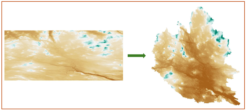
The following code converts the extended DEM to a projected Coordinate Reference System (CRS) and extracts the corresponding basin area, along with a clipped version of the DEM. The extended dem raster can be accessed from the data directory.
# converting geographic CRS to projected CRS 'EPSG:3067'
raster.crs_reprojection(
    input_file=r"C:\users\username\folder\dem_extended.tif",
    resampling_method='bilinear',
    target_crs='EPSG:3067',
    output_file=r"C:\users\username\folder\dem_extended_EPSG3067.tif",
    nodata=-9999
)

# extracting basin area and clipped DEM from extended DEM
watershed.dem_extended_area_to_basin(
    input_file=r"C:\users\username\folder\dem_extended_EPSG3067.tif",
    basin_file=r"C:\users\username\folder\basin.shp",
    output_file=r"C:\users\username\folder\dem_clipped.tif"
)
The following figure illustrates the basin extracted from the extended DEM based on the output datasets.
Hydrology
After obtaining the basin area of the DEM, the following code computes hydrological raster files for flow direction, flow accumulation, and slope. Additionally, it generates shapefiles for the stream network, main outlets, subbasins, and drainage points of the subbasins.
For the input variable outlet_type, the recommended main outlet type is single, as the multiple option can create more than one main outlet. Since the multiple option was used to derive the basin area from the extended DEM, it would be inconsistent to generate multiple main outlets within the basin area.
For the input variable tacc_type, the threshold flow accumulation type percentage considers a percentage value of the maximum flow accumulation, whereas absolute specifies the number of cells. Suppose tacc_type is set to 100 for the absolute threshold flow accumulation type, with a pixel resolution of 10 m. The threshold flow accumulation area is calculated as \(100 \times 10 \times 10 = 10000 \text{ m}^2\).
# DEM delineation
watershed.dem_delineation(
    dem_file=r"C:\users\username\folder\dem_clipped.tif",
    outlet_type='single',
    tacc_type='percentage',
    tacc_value=1,
    folder_path=r"C:\users\username\folder"
)
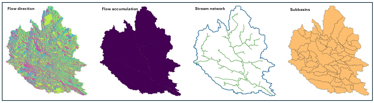
The following figure illustrates the flow direction, flow accumulation, stream network, and subbasins delived from the output datasets.
Adjacent Connectivity
Adjacent connectivity identifies the next connected segment identifiers for each stream segment in the stream network. The stream shapefile obtained in the previous section includes a column named flw_id, which contains a unique identifier for each stream segment. Using this file, the adjacent connectivty can be predicted by the follwoing code:
# adjacent downstream segment identifier
stream.connectivity_adjacent_downstream_segment(
    input_file=r"C:\users\username\folder\stream_lines.shp",
    stream_col='flw_id',
    output_file=r"C:\users\username\folder\stream_adjacent_ds_id.shp"
)
# adjacent downstream segment identifier
stream.connectivity_adjacent_upstream_segment(
    stream_file=r"C:\users\username\folder\stream_lines.shp",
    stream_col='flw_id',
    csv_file=r"C:\users\username\folder\stream_adjacent_us_id.csv"
)
Total Connectivity
Total connectivity returns dictionaries where the keys are stream segment identifiers and the values are lists representing the complete connectivity structure in the stream network. The two functions below provide connectivity in both directions: from upstream to downstream up to an outlet point, and from downstream to upstream until reaching a headwater segment.
# upstream to downstream total connectivity
stream.connectivity_upstream_to_downstream(
    stream_file=r"C:\users\username\folder\stream_lines.shp",
    stream_col='flw_id',
    json_filer"C:\users\username\folder\stream_connectivity_upstream_to_downstream.json"
)

# downstream to upstream total connectivity
stream.connectivity_downstream_to_upstream(
    stream_file=r"C:\users\username\folder\stream_lines.shp",
    stream_col='flw_id',
    json_file=r"C:\users\username\folder\stream_connectivity_downstream_to_upstream.json"
)
Remove Connectivity
To remove targeted stream segments and their corresponding upstream connections up to the headwaters, use the following code:
# removing stream segments and their upstream connectivity
stream.connectivity_remove_to_headwater(
    input_file=r"C:\users\username\folder\stream_lines.shp",
    stream_col='flw_id',
    remove_segments=[4],
    output_file=r"C:\users\username\folder\stream_connectivity_remove.shp"
)
Merge Connectivity
The following code merges split stream segments either between two junction points or from a junction point upstream until a headwater is reached. The merged segment is assigned the identifier of the most downstream segment among those being merged, and the merge information is saved to an output JSON file.
# merging split stream segments
stream.connectivity_merge_of_split_segments(
    input_file=r"C:\users\username\folder\stream_lines.shp",
    stream_col='flw_id',
    output_file=r"C:\users\username\folder\stream_split_segments_merged.shp",
    json_file=r"C:\users\username\folder\stream_split_segments_merged_information.json",
)
Junction Points
To get the junction points in a stream network, use the following code:
# junction points
stream.point_junctions(
    input_file=r"C:\users\username\folder\stream_lines.shp",
    stream_col='flw_id',
    output_file=r"C:\users\username\folder\stream_junction_points.shp"
)
Main Outlet Points
To get the main outlet points in a stream network, use the following code:
# main outlet points
stream.point_main_outlets(
    input_file=r"C:\users\username\folder\stream_lines.shp",
    output_file=r"C:\users\username\folder\stream_main_outlets.shp"
)
Headwater Points
To extract headwater points, which are the starting points of stream segments with no upstream connections, use the following code:
# headwater points
stream.point_headwaters(
    input_file=r"C:\users\username\folder\stream_lines.shp",
    stream_col='flw_id',
    output_file=r"C:\users\username\folder\stream_headwater_points.shp"
)
Stream Order
To get Strahler and Shreve order of stream segemnets, use the following code:
# Strahler order
stream.order_strahler(
    input_file=r"C:\users\username\folder\stream_lines.shp",
    stream_col='flw_id',
    output_file=r"C:\users\username\folder\strahler_order.shp"
)

# Shreve order
stream.order_shreve(
    input_file=r"C:\users\username\folder\stream_lines.shp",
    stream_col='flw_id',
    output_file=r"C:\users\username\folder\shreve_order.shp"
)